Lab 2: IMU
Setup the IMU
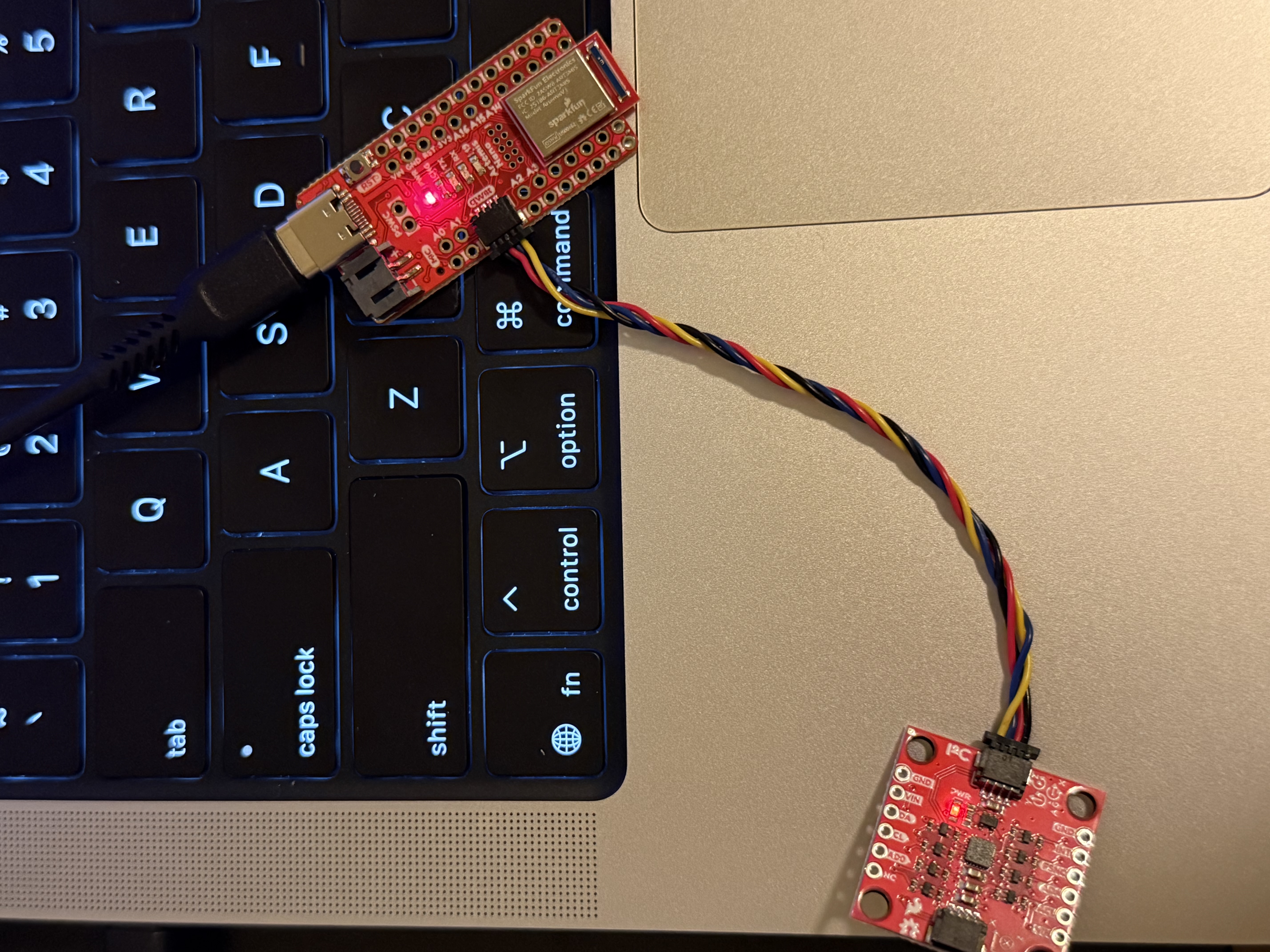
I downloaded the IMU library, and then connected the Artemis development board and the IMU to my computer, as shown in the diagram below.
After that, I ran the IMU demo in the example, and the data was printed out via the serial port, as shown in the figure.
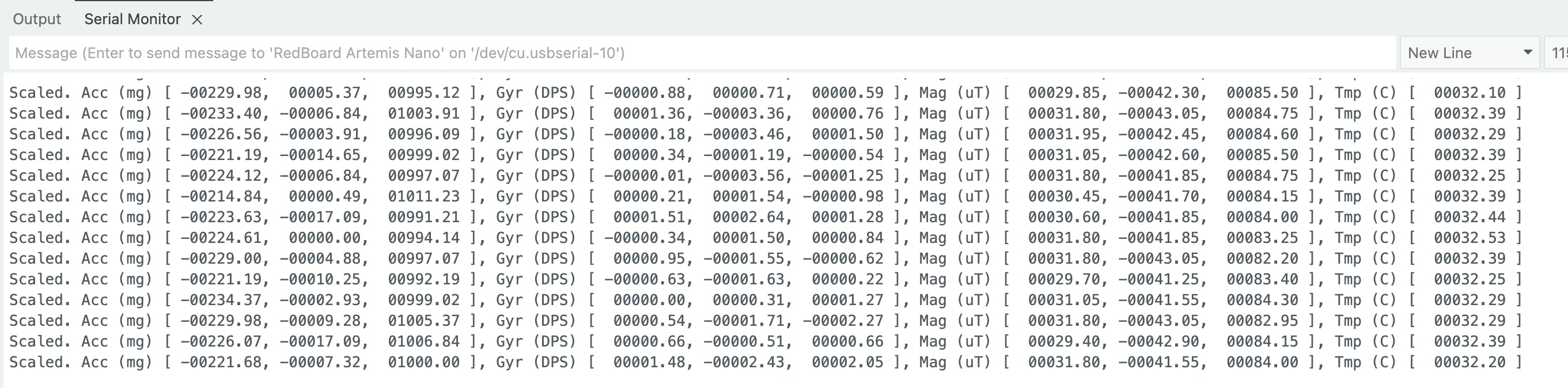
AD0_VAL represents the I2C address bit of the ICM-20948, determining which address is used for I2C; it is set to 1 by default. When the board rotates or flips, the accelerometer readings will change on the x, y, and z axes, with one axis approaching ±1 g under different orientations. When the board rotates, the gyroscope readings change, while when the board is stationary, the readings are close to 0.
Next, I wrote the development board's running indicator light, which will flash three times during program execution.
Accelerometer
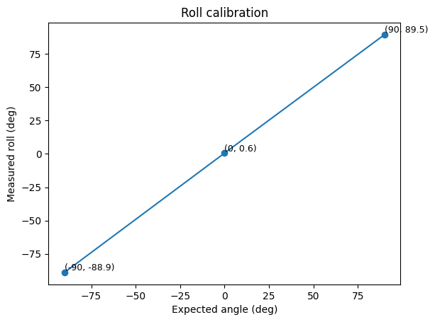
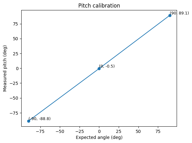
I measured the pitch and roll at three different angles: -90°, 0°, and 90°. I averaged the data from multiple sets of data printed from the serial port and finally plotted the results using two-point calibration, as shown below.
Next, I analyzed the noise during the data acquisition process. I transmitted the robot's data to my computer via Bluetooth. Using this data, I plotted the pitch and roll over time, and the presence of noise was clearly visible.
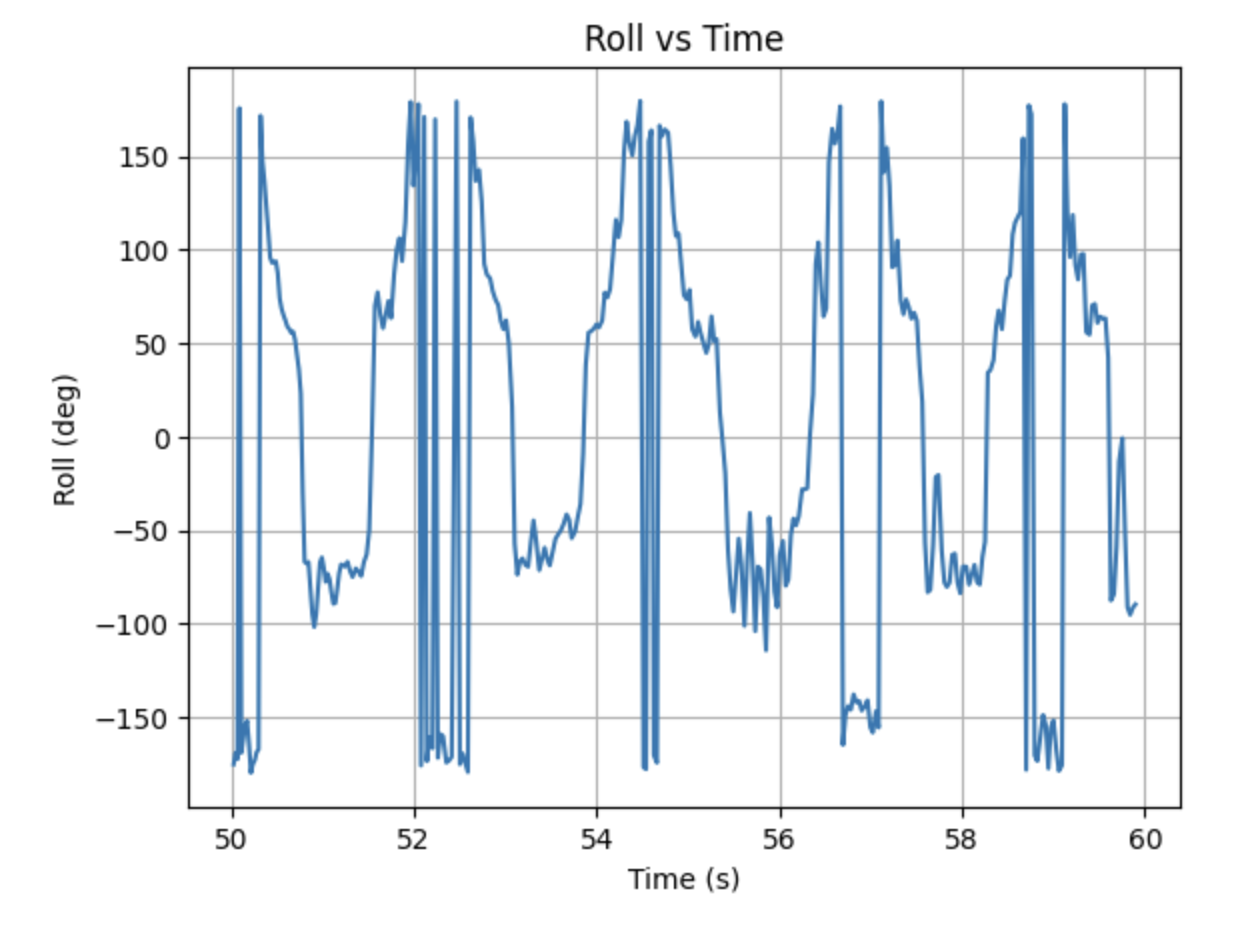
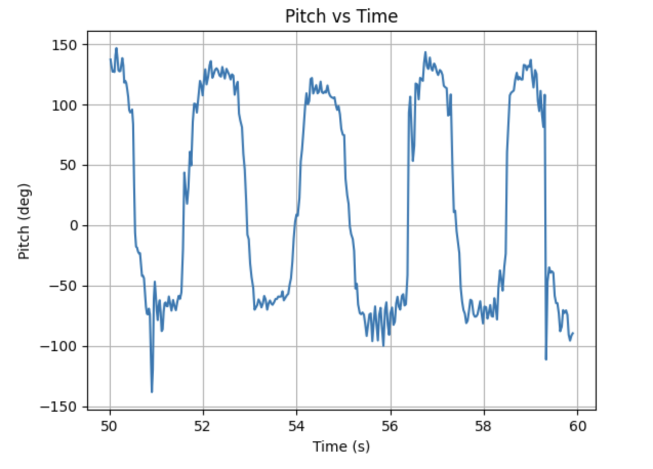
Next, I performed FFT operations on them respectively, and the extracted spectra are shown below. It can be seen that the amplitude drops sharply after 2Hz, indicating that the energy is concentrated within 2Hz. After 2Hz, there is high-frequency noise. Therefore, the cutoff frequency is set to 2Hz.
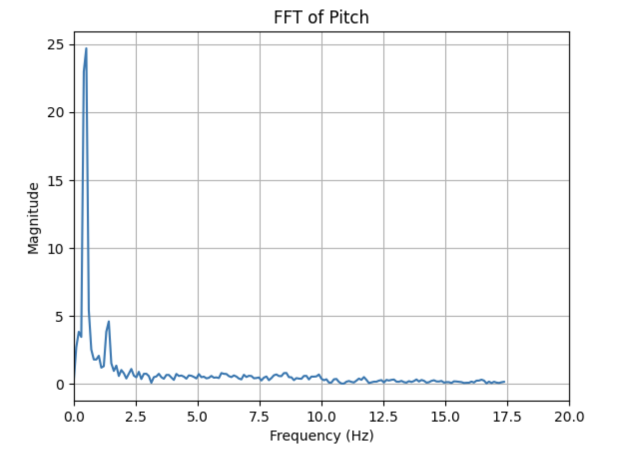
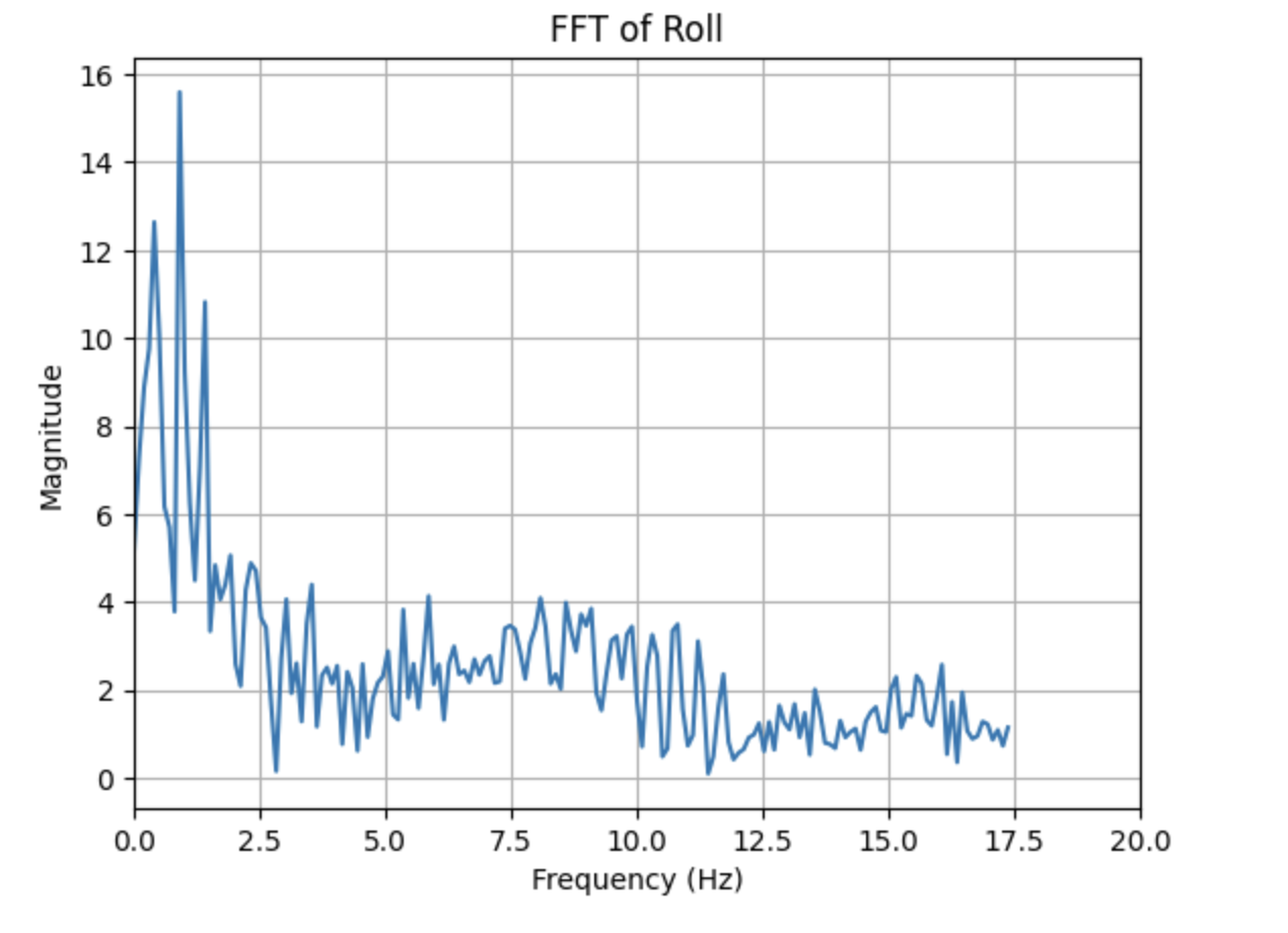
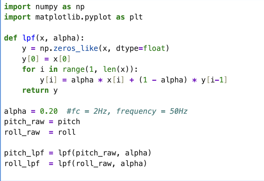
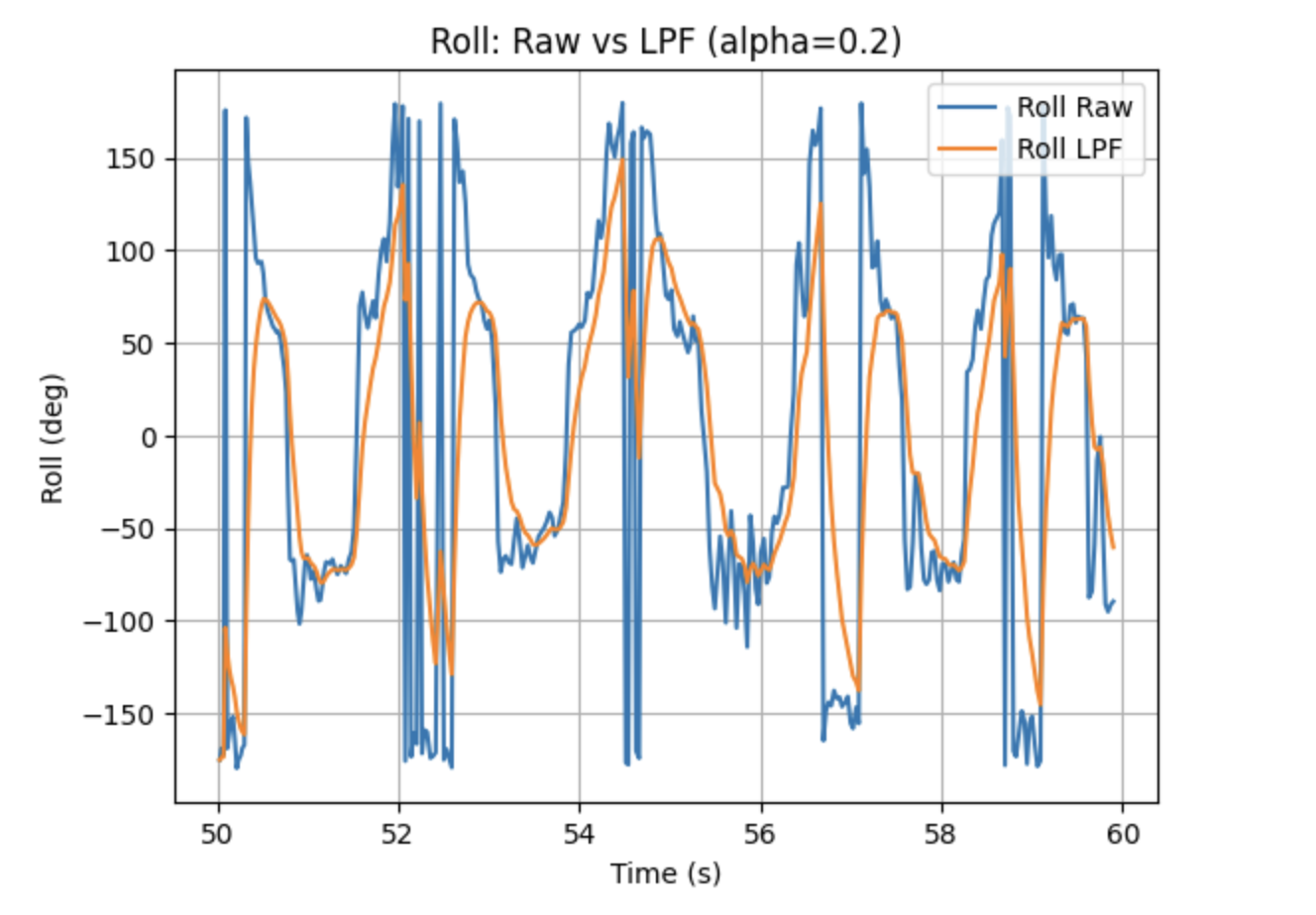
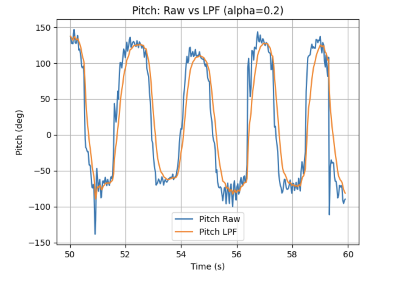
Based on this cutoff frequency, I designed a low-pass filter. In the program, I set the frequency to 50Hz. The code and filtering effect are shown below. As we can see, the signal becomes much smoother.
Gyroscope
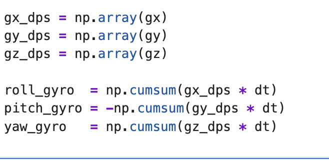
Based on the formulas learned in class, the code for calculating pitch, roll, and yaw using a gyroscope is shown below.
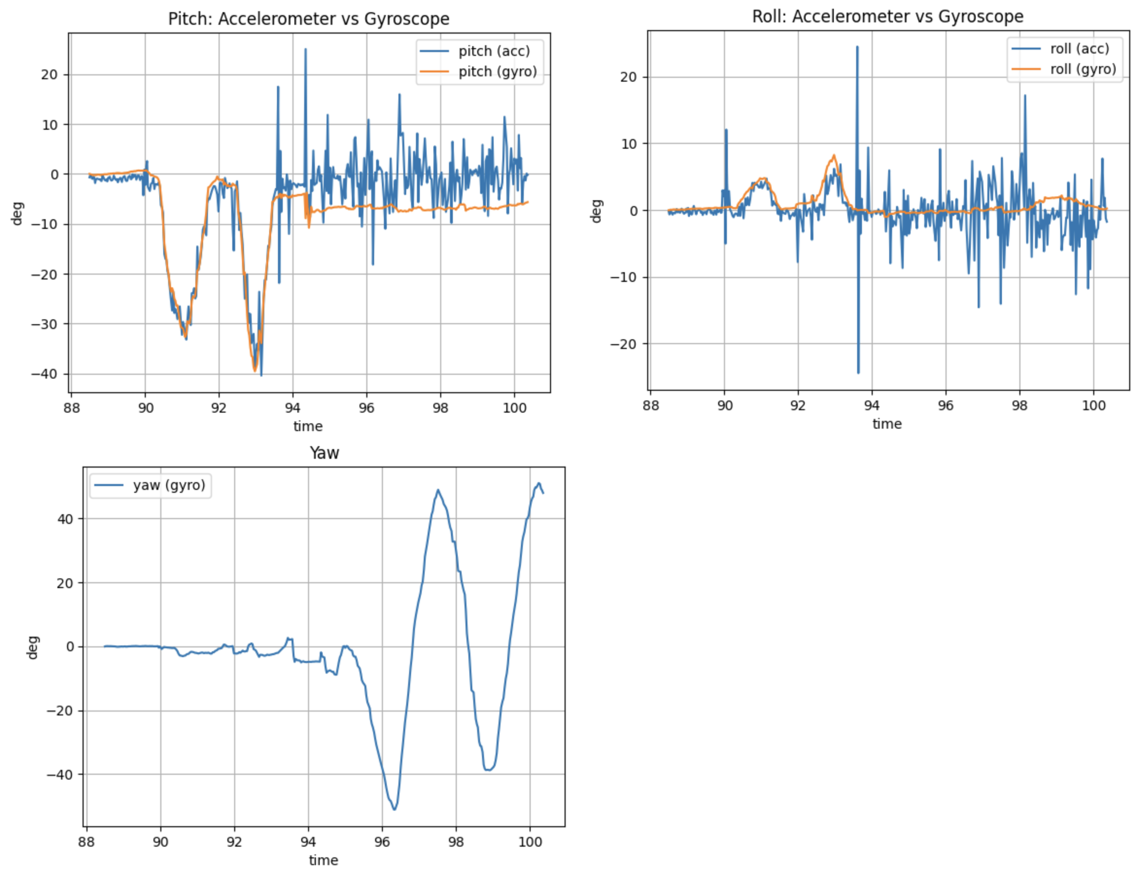
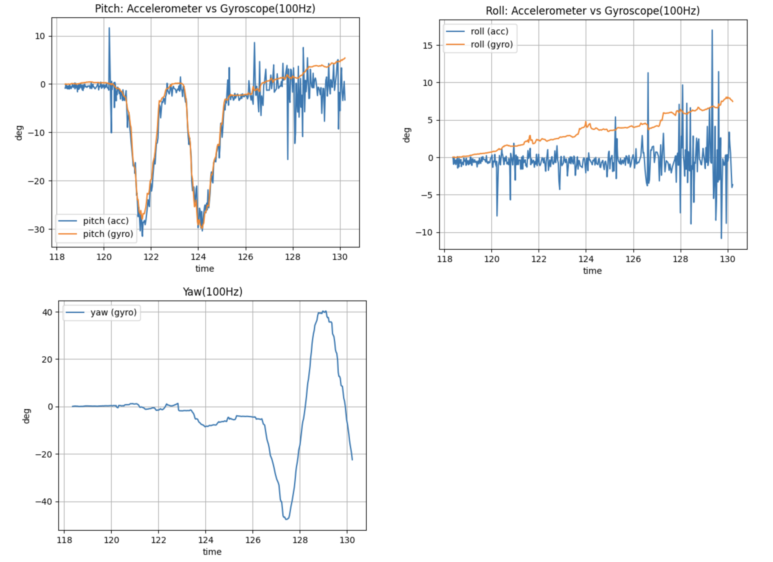
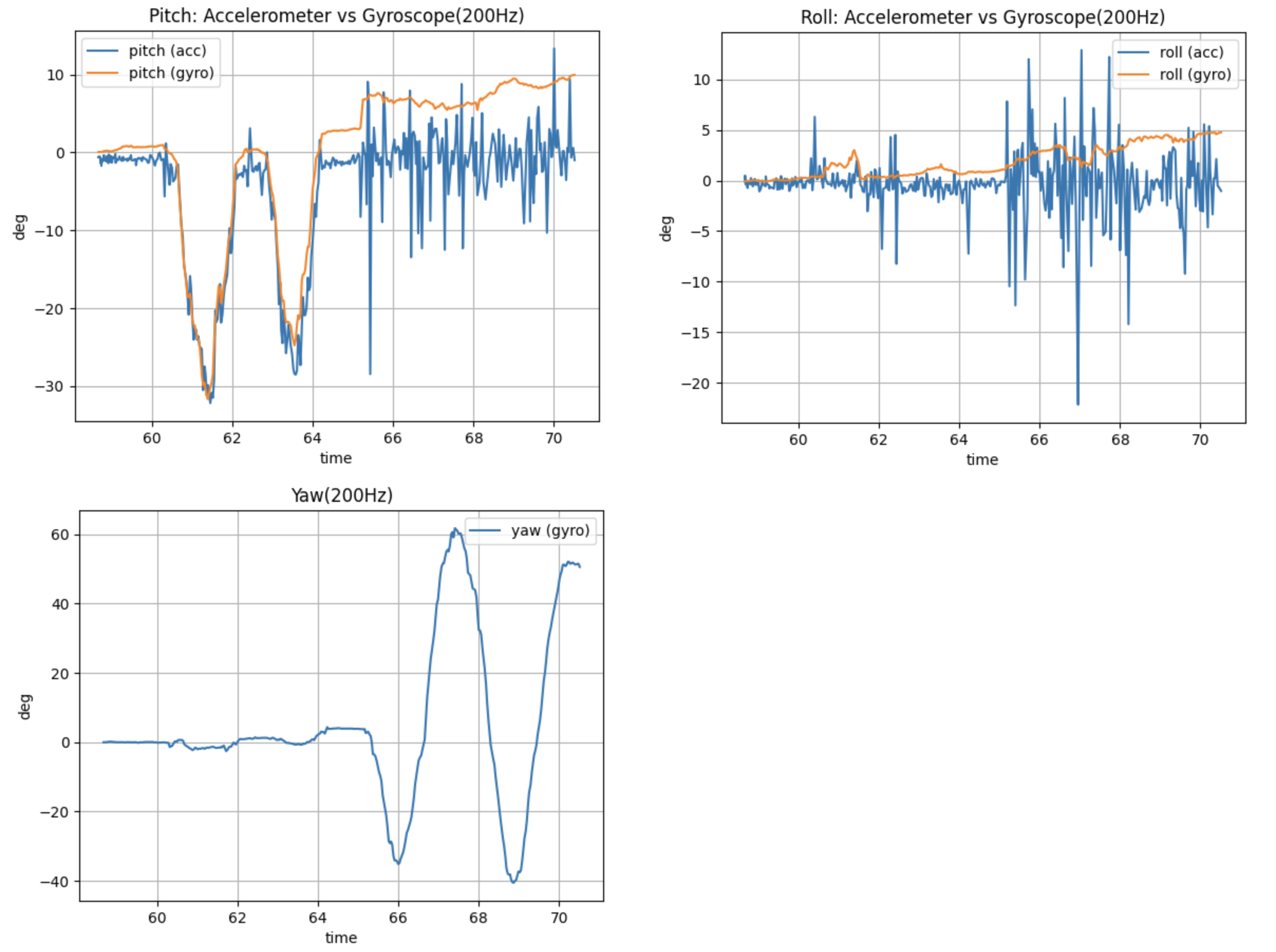
By changing the acquisition frequency, the following images show pitch, roll, and yaw data acquired using an accelerometer and gyroscope at different frequencies. The comparison revealed that the accelerometer can reflect the true attitude, but it is more sensitive to noise and there are obvious jitters in the curve; while the data obtained by integrating the gyroscope is smoother in the short term, but will drift significantly over time. As the sampling frequency increases, the details of attitude changes are more fully reflected, and the curves become smoother, but high-frequency noise also becomes more noticeable.
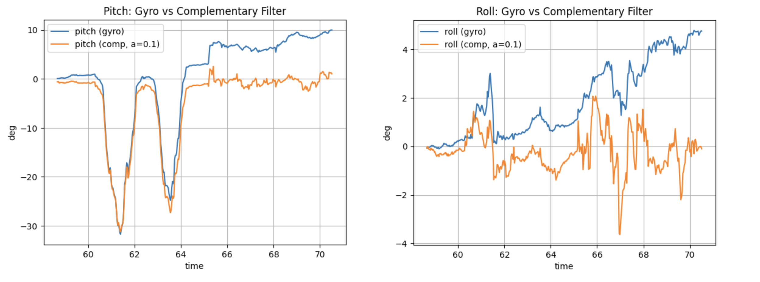
Next, I used the complementary filter I learned in class to combine the data from the gyroscope and accelerometer. I found that the results were more stable and the high-frequency jitter was significantly reduced.

Sample Data
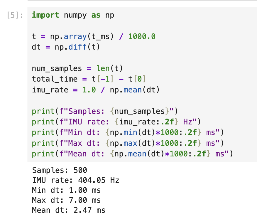
To accelerate the execution speed of the main loop, a blocking approach was not used to wait for IMU data to be ready. Instead, the IMU data was checked for readiness in each iteration of the main loop. The results are shown below: a total of 500 samples were collected, with an average sampling interval of 2.47 ms and a corresponding average sampling rate of approximately 404 Hz. The minimum and maximum sampling intervals were 1 ms and 7 ms, respectively. The results indicate that the execution speed of Artemis' main loop is significantly faster than the speed at which the IMU generates new data.
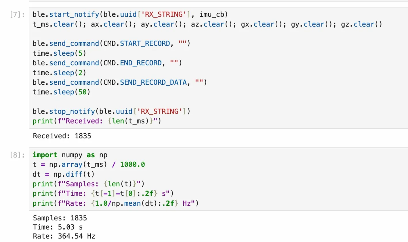
Next, I stored the timestamped IMU data into an array. I added three new commands: START_RECORD, END_RECORD, and SEND_RECORD_DATA, which are responsible for starting recording, stopping recording, and sending data to the computer, respectively. The result is shown in the figure below, proving that five seconds of data can be collected.
Separate arrays were chosen to store the data for easier access. An unsigned long data type is used for time, and float is used for IMU data, as this matches the corresponding libraries. Global variables occupy 117KB of memory (29%), leaving 275KB of memory available.
